You define the headway of a line using the time profile attribute Headway (User Manual: Headway-based assignment: Basis tab).
If you want to model a time-dynamic headway, you can use a time interval set that has been attributed as a headway time interval set. Its time intervals are available as subattributes of the headway.
In the case of a time-dynamic headway, the headway is specified separately according to time intervals. This allows you to model that transport supply varies during the assignment period, for example, that demand is higher during the morning rush hour.
If no information on the headway is specified, but a timetable with vehicle journeys is available, Visum can determine the headway. You can determine it using a special function or in the headway-based assignment. The following options are available:
- from the mean headway according to the timetable
- from the mean wait time according to the timetable (default setting)
From mean headway according to timetable
Visum can also automatically calculate the headway from the timetable of the time profile. For that purpose, the number of departures n is determined for each time interval l = [a,b) within the assignment time period. The headway results as the quotient.

In the case of networks with short headways and sufficiently broad time intervals, this simplified approximation is acceptable. Generally speaking, however, this approach is problematic for two reasons.
On the one hand, the definition is too sensitive to shiftings of individual departures across the interval limits. This will cause discontinuities in the result. This problem always occurs if the real headway of a PT line is no divisor of the length of the demand time interval. For a line with a 40-minute headway, for example, and the time interval l = [06:00 a.m., 07:00 a.m.), different headways are calculated for the particular departure times (Table 179).
On the other hand, this approach cannot reflect the following fact: For the passenger who arrives at random, trips spread evenly throughout the time interval generally mean less wait time than trips that are piled up. The following third definition, therefore, is used as the default setting for the headway-based procedure.
From mean wait time according to timetable
The headway τa,b of a line is defined as double the expected wait time for the next departure of the line in the case of random access in the time interval [a,b).
Fl = {x1, x2, ..., xn} is the set of departure times of the line in interval l = [a,b). The first departure after time b is indicated as x‘. Since such a departure does not have to exist or can occur later, the fictitious departure x‘‘ = x1 + (b-a), which results from the cyclical continuation of the timetable in l, is also considered. For the calculation of the wait time at the end of l the departure xn+1 = min{x‘,x‘‘} is used.
The headway is then defined as follows.
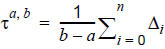
Here applies:  ,
,  and
and 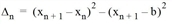 to the remaining i ∈ {1, ..., n-1}. ∆Ii is in each case the expected wait time in a sub-interval.
If you now look again at the example with the 40-minute headway and the interval l = [06:00,07:00), you get a much more balanced picture.
Using the example in the first row, the calculation can be briefly explained as follows.
In this case n = 1, x1 = 06:35 and x2 = 07:15 apply.
Therefore follows
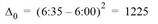 and
and 
Overall this results in 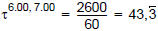 minutes.
Compared to the case of the naive approach  , this example shows that the calculated values vary far less when shifting the specific departure times.
